Time-Varying Exposure
In this section, we will go through some methods to estimate the average causal effect of a time-varying treatment / exposure on a specific outcome. The key problem we must overcome is time-varying confounding. Time-varying confounders are both a mediator and a confounder, depending on the causal path. As such, conditional models will not correctly estimate the causal effects with time-varying confounders. We need to use special methods to account for time-varying confounding. We will focus on time-to-event and longitudinal data separately.
To help solidify understanding, consider the following causal diagram, where subscripts are used to indicate time
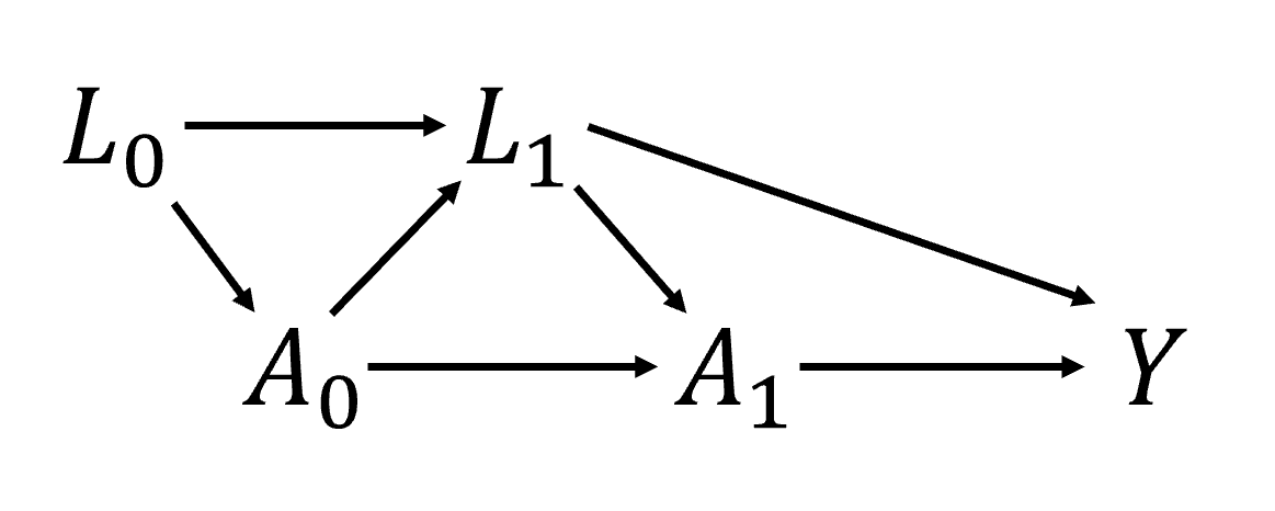
If we are interested in the effect of \(A\) (not only \(A_0\)), then we need to account for confounding variables. \(L_0\) is easy, since we know we can condition on this variable safely. The problem comes with \(L_1\). On the \(A_0\) causal path to \(Y\), \(L_1\) is a mediator. However, on the \(A_1\) to \(Y\) causal path, \(L_1\) is a confounder. Therefore, we need to simultaneously condition on \(L_1\), while also not condition on it. We can’t do that, so we are damned if we do and damned if we don’t.
Not all hope is lost. James Robins developed his “g-methods” (g-formula, IPTW, g-estimation) for this exact problem. These methods allows us to account for confounding by \(L_1\), but do not require conditioning on any variables. Instead the g-methods provide marginal estimates rather than conditional. I introduced g-methods in the baseline exposure setting, but time-varying exposure is where these methods really shine.
We will assume conditional mean exchangeability, causal consistency, and positivity throughout. These assumptions allow us to go from our observed data to potential outcomes. See Hernan and Robins for further details on these assumptions and the g-methods in general.
This section is divided into two scenarios; time-to-event and longitudinal data. For time-to-event, I mean that we have data collected on the exact time of the event. For the g-methods, we will coarsen this data to discrete time, but this is only necessary since we have finite data. As for longitudinal, I mean that our input data is already coarsened. The data comes from follow-ups at constant intervals. The event at the follow-up visit happened some time between the previous visit and the current visit. I draw this distinction, since some approaches for estimation work better in one scenario over the other.
Time-to-Event Data
We will start with estimating the average causal effect of ART on mortality, assuming that once someone is treated with ART, they remain on treatment (I will refer to as the intent-to-treat assumption in this tutorial). We will set up the environment with the following code
import numpy as np
import pandas as pd
from lifelines import KaplanMeierFitter

from zepid import load_sample_data, spline
from zepid.causal.gformula import MonteCarloGFormula
from zepid.causal.ipw import IPTW, IPCW

df = load_sample_data(timevary=True)

# Background variable preparations
df['lag_art'] = df['art'].shift(1)
df['lag_art'] = np.where(df.groupby('id').cumcount() == 0, 0, df['lag_art'])
df['lag_cd4'] = df['cd4'].shift(1)
df['lag_cd4'] = np.where(df.groupby('id').cumcount() == 0, df['cd40'], df['lag_cd4'])
df['lag_dvl'] = df['dvl'].shift(1)
df['lag_dvl'] = np.where(df.groupby('id').cumcount() == 0, df['dvl0'], df['lag_dvl'])
df[['age_rs0', 'age_rs1', 'age_rs2']] = spline(df, 'age0', n_knots=4, term=2, restricted=True)  # age spline
df['cd40_sq'] = df['cd40'] ** 2  # cd4 baseline cubic
df['cd40_cu'] = df['cd40'] ** 3
df['cd4_sq'] = df['cd4'] ** 2  # cd4 current cubic
df['cd4_cu'] = df['cd4'] ** 3
df['enter_sq'] = df['enter'] ** 2  # entry time cubic
df['enter_cu'] = df['enter'] ** 3
We will assume conditional exchangeability by age (continuous), gender (male / female), baseline CD4 T-cell count (continuous), and baseline detectable viral load (yes / no), CD4 T-cell count (continuous), detectable viral load (yes / no), and previous ART treatment. CD4 T-cell count and detectable viral load are time-varying confounders in this example.
Our set of confounders for conditional exchangeability is quite large and includes some continuous variables. Therefore, we will use parametric models (for the most part). As a result, we assume that our models are correctly specified, in addition to the above assumptions.
Monte-Carlo g-formula
The first option is to use the Monte-Carlo g-formula. This approach works by estimating pooled logistic regression models for each time-varying variable (treatment, outcome, time-varying confounding). We then sample the population from baseline and predict individuals’ time-varying variables going forward in time. We use Monte Carlo re-sampling to reduce simulation error of the outcomes.
To begin, we initialize the Monte-Carlo g-formula with
mcgf = MonteCarloGFormula(df,  # Data set
                          idvar='id',  # ID variable
                          exposure='art',  # Exposure
                          outcome='dead',  # Outcome
                          time_in='enter',  # Start of study period
                          time_out='out')  # End of time per study period
We then specify models for each of our time-varying variables (ART, death, CD4 T-cell count, detectable viral load). Additionally, we will specify a model for censoring. Below is example code for this procedure
# Pooled Logistic Model: Treatment
exp_m = ('male + age0 + age_rs0 + age_rs1 + age_rs2 + cd40 + cd40_sq + cd40_cu + dvl0 + '
         'cd4 + cd4_sq + cd4_cu + dvl + enter + enter_sq + enter_cu')
mcgf.exposure_model(exp_m,
                    restriction="g['lag_art']==0")  # Restricts to only untreated (for ITT assumption)

# Pooled Logistic Model: Outcome
out_m = ('art + male + age0 + age_rs0 + age_rs1 + age_rs2 + cd40 + cd40_sq + cd40_cu + dvl0 + '
         'cd4 + cd4_sq + cd4_cu + dvl + enter + enter_sq + enter_cu')
mcgf.outcome_model(out_m,
                   restriction="g['drop']==0")  # Restricting to only uncensored individuals

# Pooled Logistic Model: Detectable viral load
dvl_m = ('male + age0 + age_rs0 + age_rs1 + age_rs2 + cd40 + cd40_sq + cd40_cu + dvl0 + '
         'lag_cd4 + lag_dvl + lag_art + enter + enter_sq + enter_cu')
mcgf.add_covariate_model(label=1,  # Order to fit time-varying models in
                         covariate='dvl',  # Time-varying confounder
                         model=dvl_m,
                         var_type='binary')  # Variable type

# Pooled Logistic Model: CD4 T-cell count
cd4_m = ('male + age0 + age_rs0 + age_rs1 + age_rs2 +  cd40 + cd40_sq + cd40_cu + dvl0 + lag_cd4 + '
         'lag_dvl + lag_art + enter + enter_sq + enter_cu')
cd4_recode_scheme = ("g['cd4'] = np.maximum(g['cd4'], 1);"
                     "g['cd4_sq'] = g['cd4']**2;"
                     "g['cd4_cu'] = g['cd4']**3")
mcgf.add_covariate_model(label=2,  # Order to fit time-varying models in
                         covariate='cd4',  # Time-varying confounder
                         model=cd4_m,
                         recode=cd4_recode_scheme,  # Recoding process to use for each iteraction of MCMC
                         var_type='continuous')  # Variable type

# Pooled Logistic Model: Censoring
cens_m = ("male + age0 + age_rs0 + age_rs1 + age_rs2 +  cd40 + cd40_sq + cd40_cu + dvl0 + lag_cd4 + " +
          "lag_dvl + lag_art + enter + enter_sq + enter_cu")
mcgf.censoring_model(cens_m)
After our models are specified, we can now predict the outcome plans under our treatment plan. To start, we will compare to the natural course. The natural course is the world observed as it is. Since we are relying on the ITT assumption, we will use the custom treatment option to fit the natural course. Below is code to estimate the natural course under the ITT assumption
mcgf.fit(treatment="((g['art']==1) | (g['lag_art']==1))",  # Treatment plan
         lags={'art': 'lag_art',  # Lagged variables to create each loop
               'cd4': 'lag_cd4',
               'dvl': 'lag_dvl'},
         in_recode=("g['enter_sq'] = g['enter']**2;"  # Recode statement to execute at the start
                    "g['enter_cu'] = g['enter']**3"),
         sample=20000)  # Number of resamples from population (should be large number)
Afterwards, we can generate a plot of the risk curves.
# Accessing predicted outcome values
gf = mcgf.predicted_outcomes

# Fitting Kaplan Meier to Natural Course
kmn = KaplanMeierFitter()
kmn.fit(durations=gfs['out'], event_observed=gfs['dead'])

# Fitting Kaplan Meier to Observed Data
kmo = KaplanMeierFitter()
kmo.fit(durations=df['out'], event_observed=df['dead'], entry=df['enter'])

# Plotting risk functions
plt.step(kmn.event_table.index, 1 - kmn.survival_function_, c='k', where='post', label='Natural')
plt.step(kmo.event_table.index, 1 - kmo.survival_function_, c='gray', where='post', label='True')
plt.legend()
plt.show()
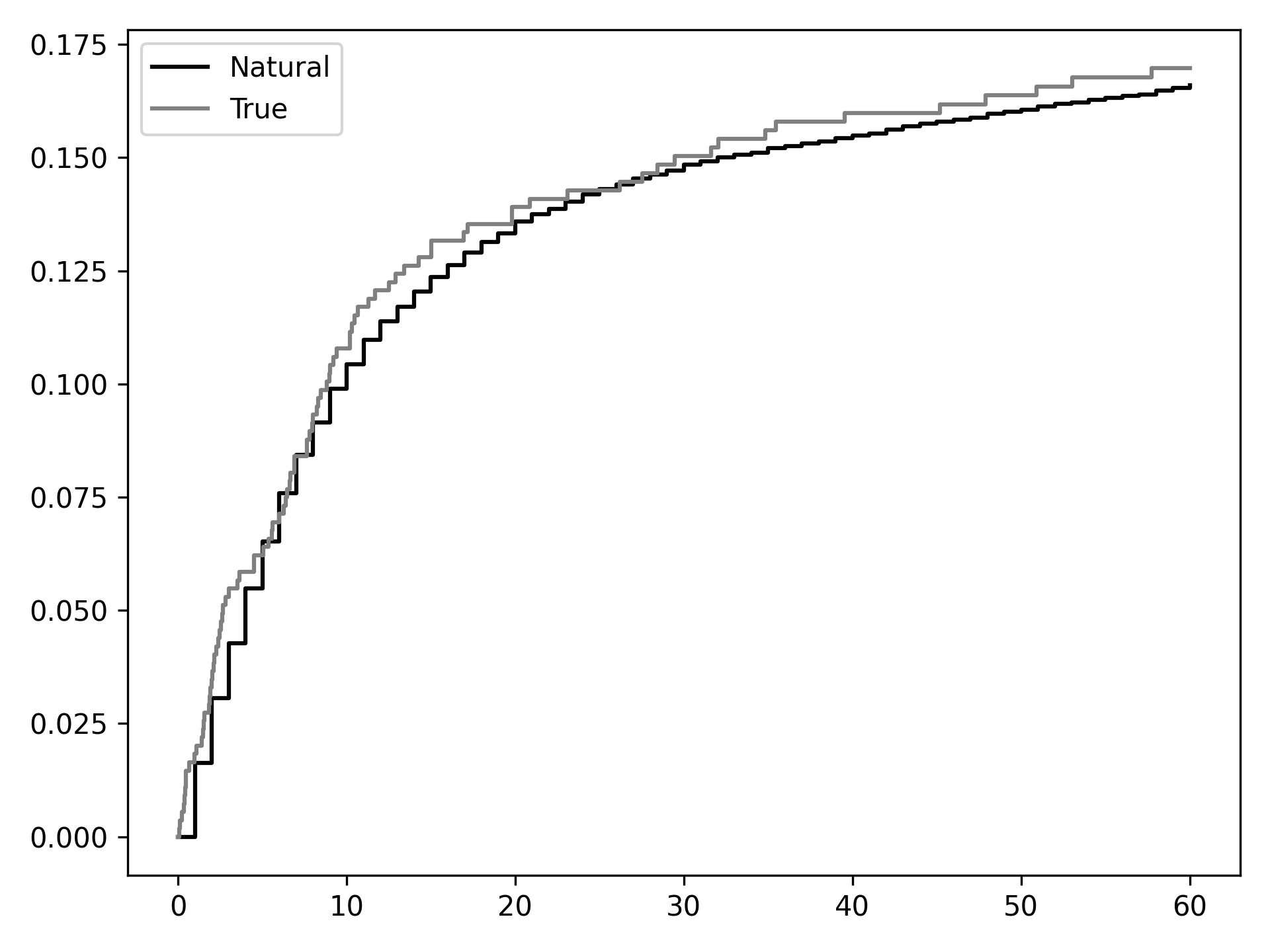
From this we can see that out natural course predictions (black) follow the observed data pretty well (gray). Note: this does not mean that our models are correctly specified. Rather it only means they may not be incorrectly specified. Sadly, there is no way to know that all our models are correctly specified… We may take some comfort that our curves largely overlap, but do not take this for granted.
We can now estimate the counterfactual outcomes under various treatment plans. In the following code, we will estimate the outcomes under treat-all plan, treat-none plan, and treat only once CD4 T-cell count drops below 200.
# Treat-all plan
mcgf.fit(treatment="all",
         lags={'art': 'lag_art',
               'cd4': 'lag_cd4',
               'dvl': 'lag_dvl'},
         in_recode=("g['enter_sq'] = g['enter']**2;"
                    "g['enter_cu'] = g['enter']**3"),
         sample=20000)
g_all = mcgf.predicted_outcomes

# Treat-none plan
mcgf.fit(treatment="none",
         lags={'art': 'lag_art',
               'cd4': 'lag_cd4',
               'dvl': 'lag_dvl'},
         in_recode=("g['enter_sq'] = g['enter']**2;"
                    "g['enter_cu'] = g['enter']**3"),
         sample=20000)
g_none = mcgf.predicted_outcomes

# Custom treatment plan
mcgf.fit(treatment="g['cd4'] <= 200",
         lags={'art': 'lag_art',
               'cd4': 'lag_cd4',
               'dvl': 'lag_dvl'},
         in_recode=("g['enter_sq'] = g['enter']**2;"
                    "g['enter_cu'] = g['enter']**3"),
         sample=20000,
         t_max=None)
g_cd4 = mcgf.predicted_outcomes

# Risk curve under treat-all
gfs = g_all.loc[g_all['uid_g_zepid'] != g_all['uid_g_zepid'].shift(-1)].copy()
kma = KaplanMeierFitter()
kma.fit(durations=gfs['out'], event_observed=gfs['dead'])

# Risk curve under treat-all
gfs = g_none.loc[g_none['uid_g_zepid'] != g_none['uid_g_zepid'].shift(-1)].copy()
kmn = KaplanMeierFitter()
kmn.fit(durations=gfs['out'], event_observed=gfs['dead'])

# Risk curve under treat-all
gfs = g_cd4.loc[g_cd4['uid_g_zepid'] != g_cd4['uid_g_zepid'].shift(-1)].copy()
kmc = KaplanMeierFitter()
kmc.fit(durations=gfs['out'], event_observed=gfs['dead'])

# Plotting risk functions
plt.step(kma.event_table.index, 1 - kma.survival_function_, c='blue', where='post', label='All')
plt.step(kmn.event_table.index, 1 - kmn.survival_function_, c='red', where='post', label='None')
plt.step(kmc.event_table.index, 1 - kmc.survival_function_, c='green', where='post', label='CD4 < 200')
plt.legend()
plt.show()
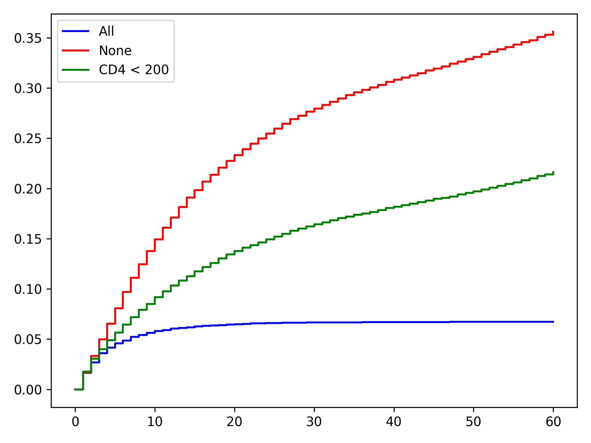
From these results, we can see that the treat-all plan reduces the probability of death across all time points. Importantly, the treat-all plan outperforms the custom treatment plan. Based on this result, we would recommend that all HIV-infected individuals receive ART treatment as soon as they are diagnosed.
To obtain confidence intervals, nonparametric bootstrapping should be used. Take note that this will take awhile to finish (especially if a high number of resamples are used). As it stands, MonteCarloGFormula is slow, and future work is to try to optimize the Monte Carlo procedure (specifically with some large matrix multiplications)
Marginal Structural Model
We can also use inverse probability of treatment weights to estimate a marginal structural model for time-varying
treatments. Similar to the Monte-Carlo g-formula, we will rely on the same ITT assumption previous described. To
calculate the corresponding IPTW, we will use IPTW again. Since we will need to do further manipulation of the
predicted probabilities, we will have IPTW return the predicted probabilities of the denominator and numerator,
respectively. We do this through the following code
# Specifying models
modeln = 'enter + enter_q + enter_c'
modeld = ('enter + enter_q + enter_c + male + age0 + age0_q + age0_c + dvl0 + cd40 + '
          'cd40_q + cd40_c + dvl + cd4 + cd4_q + cd4_c')

# Restricting to only the previously untreated data
dfs = df.loc[df['lagart']==0].copy()

# Calculating probabilities for IPTW
ipt = IPTW(dfs, treatment='art')
ipt.regression_models(model_denominator=modeld, model_numerator=modeln)
ipt.fit()

# Extracting probabilities for later manipulation
df['p_denom'] = ipt.ProbabilityDenominator
df['p_numer'] = ipt.ProbabilityNumerator
Note: you should only use stabilized weights for time-varying treatments. Unstabilized weights can have poor performance
We now need to do some further manipulation of the weights
#Condition 1: First record weight is 1
cond1 = (df.groupby('id').cumcount() == 0)
df['p_denom'] = np.where(cond1, 1, df['p_denom']) #Setting first visit to Pr(...) = 1
df['p_numer'] = np.where(cond1, 1, df['p_numer'])
df['ip_denom'] = np.where(cond1, 1, (1-df['p_denom']))
df['ip_numer'] = np.where(cond1, 1, (1-df['p_numer']))
df['den'] = np.where(cond1, df['p_denom'], np.nan)
df['num'] = np.where(cond1, df['p_numer'], np.nan)

#Condition 2: Records before ART initiation
cond2 = ((df['lagart']==0) & (df['art']==0) & (df.groupby('id').cumcount() != 0))
df['num'] = np.where(cond2, df.groupby('id')['ip_numer'].cumprod(), df['num'])
df['den'] = np.where(cond2, df.groupby('id')['ip_denom'].cumprod(), df['den'])

#Condition 3: Records at ART initiation
cond3 = ((df['lagart']==0) & (df['art']==1) & (df.groupby('id').cumcount() != 0))
df['num'] = np.where(cond3, df['num'].shift(1)*(df['p_numer']), df['num'])
df['den'] = np.where(cond3, df['den'].shift(1)*(df['p_denom']), df['den'])

#Condition 4: Records after ART initiation
df['num'] = df['num'].ffill()
df['den'] = df['den'].ffill()

#Calculating weights
df['w'] = df['num'] / df['den']
After calculating our weights, we can estimate the risk functions via a weighted Kaplan Meier. Note that
lifelines version will need to be 0.14.5 or greater. The following code will generate our risk function plot
kme = KaplanMeierFitter()
dfe = df.loc[df['art']==1].copy()
kme.fit(dfe['out'],event_observed=dfe['dead'],entry=dfe['enter'],weights=dfe['w'])

kmu = KaplanMeierFitter()
dfu = df.loc[df['art']==0].copy()
kmu.fit(dfu['out'],event_observed=dfu['dead'],entry=dfu['enter'],weights=dfu['w'])

plt.step(kme.event_table.index,1 - kme.survival_function_,c='b',label='ART')
plt.step(kmu.event_table.index,1 - kmu.survival_function_,c='r',label='no ART')
plt.show()
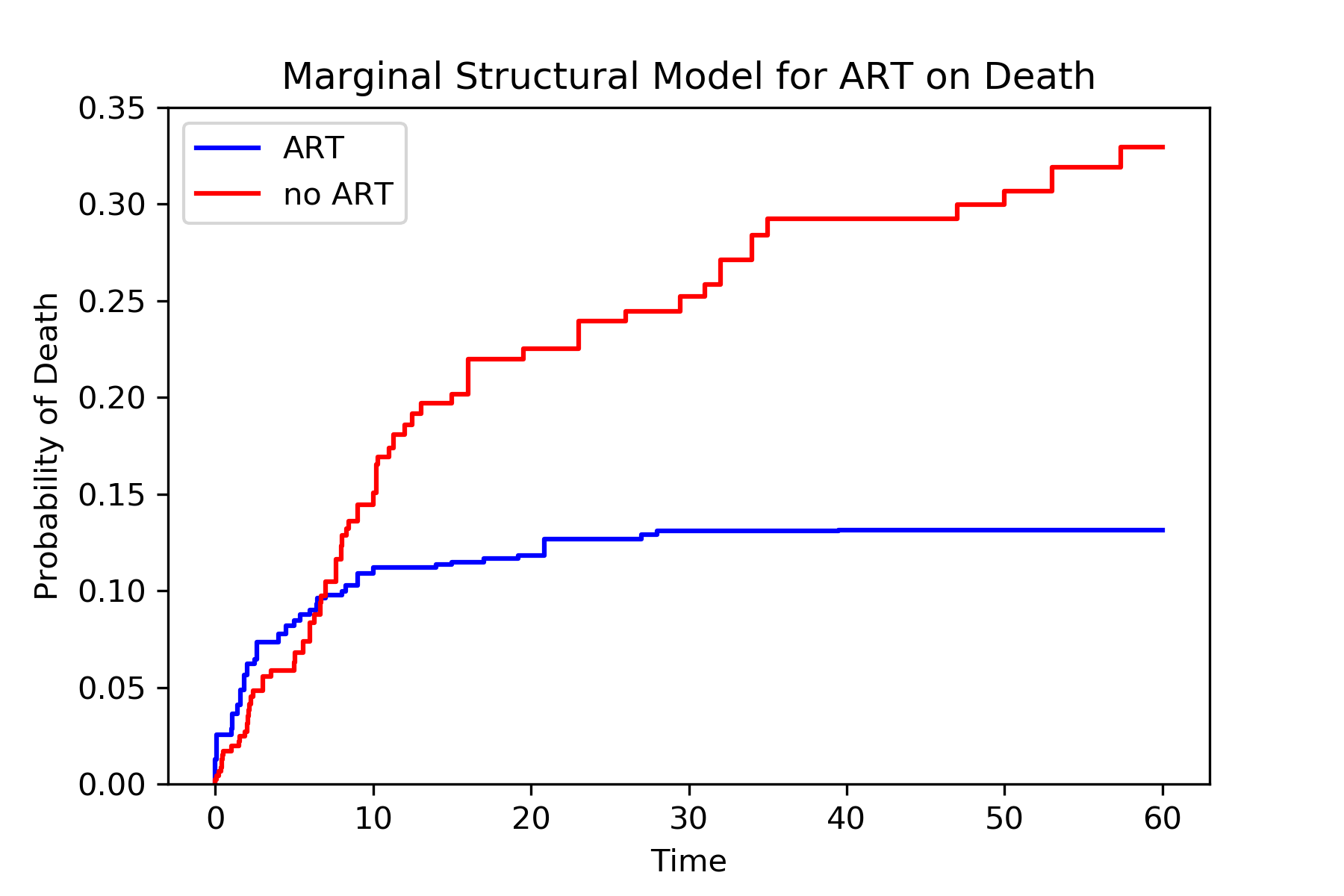
Similarly, we see the treat-all plan is better than the never-treat plan. We see a discrepancy between the two approaches during the early times (weeks less than 5). Note that we did not account for informative censoring. To account for informative censoring, we could use inverse probability of censoring weights. See the Missing Data tutorial for further details.
Longitudinal Data
We will use a different simulated data set within zEpid for this section. This data is longitudinal data simulated for demonstrative purposes. This data set is in a wide-format, such that each row is a single person and columns are variables measured at specific time points. Note: this format is distinct from the time-to-event data, which was in a long format. Below is code to load this data set
from zepid import load_longitudinal_data
df = load_longitudinal_data()
In this data, we have outcomes measured at three time points. Additionally, we have treatments (A), time-varying confounder (L), and a baseline confounder (W) measured in our data. We will assume exchangeability (sometimes also referred to as sequential ignorability) for the effect of A on Y by L and W.
Iterative Conditional g-formula
The iterative conditional g-formula is an alternative to the Monte-Carlo estimation procedure, as detailed in the previous sections. While the Monte-Carlo g-formula requires that we specify a parametric regression model for all time-varying variables, the iterative conditional approach only requires that we specify an outcome regression model. This drastically cuts down on the potential for model misspecification. However, we no longer use a pooled logistic regression model, so the iterative conditional g-formula does not estimate nicely in sparse survival data (in my experience).
The iterative conditional procedure works like the following. Starting at the last observed time, we fit our specified outcome model. From this model, we predict the probability of the outcome under observed treatment (\(\hat{Q}\)) and under the counterfactual treatment of interest (\(Q^*\)). Next, we move to the previous time point. For those who were observed at the last time point, we use their \(\hat{Q}\) as their outcome. If they were not observed at the furtherest time point, we use their observed \(Y\) instead. We repeat the process of model fitting. We then repeat this whole procedure (hence “iterative” conditionals) until we end up at the origin. Now our predicted \(Q^*\) value is the counterfactual mean under the specified treatment plan
The following is code to use the iterative conditional process. We will start with estimating the counterfactual mean under a treat-all strategy for t=3.
icgf = IterativeCondGFormula(df, exposures=['A1', 'A2', 'A3'], outcomes=['Y1', 'Y2', 'Y3'])

# Specifying regression models for each treatment-outcome pair
icgf.outcome_model(models=['A1 + L1',
                           'A2 + A1 + L2',
                           'A3 + A2 + L3'],
                   print_results=False)

# Estimating marginal ‘Y3’ under treat-all at every time
icgf.fit(treatments=[1, 1, 1])
r_all = icgf.marginal_outcome
r_all is the overall risk of Y at time 3 under a treat-all at all time points strategy. This value was 0.433. We can estimate the overall risk of Y at time 3 under a treat-none strategy by running
icgf.fit(treatments=[0, 0, 0])
r_non = icgf.marginal_outcome

print('RD =', r_all - r_non)
We can interpret our estimated risk difference as: the risk of Y at time 3 under a treat-all strategy was 19.5% points lower than under a treat-none strategy. We can make further comparisons between treatment plans by changing the treatments argument. Below is an example where treatment is only given a baseline
icgf.fit(treatments=[1, 0, 0])
The estimated risk under this treatment strategy is 0.547. To estimate Y at t=2, we use a similar process as above but limit our data to Y2. Below is an example of estimating Y at t=2 for a treat-all strategy
icgf = IterativeCondGFormula(df, exposures=['A1', 'A2'], outcomes=['Y1', 'Y2'])
icgf.outcome_model(models=['A1 + L1',
                           'A2 + A1 + L2'],
                   print_results=False)
icgf.fit(treatments=[1, 1])
The estimate risk of Y at t=2 under a treat-all strategy was 0.350. The above process can be repeated for all observation times in a wide data set. For calculation of confidence intervals, a non-parametric bootstrapping procedure should be used.
Marginal Structural Model
We can also use inverse probability weights to estimate a marginal structural model. Easier implementation of this estimation will be added later.
Longitudinal TMLE
In a future update, the longitudinal targeted maximum likelihood estimator will be added.
G-estimation
Currently, g-estimation of structural nested models for time-varying exposures is not implemented. I plan to add AFT estimation procedures in a future update
Summary
G-methods allow us to answer more complex questions than standard methods. With these tools, we can start to ask questions about ideal treatment strategies. See further tutorials at this GitHub repo for further examples